GoodVibes
Here is the GoodVibes GitHub Page
Here is the GoodVibes Publication
Installation
Version 4.2.0 is most up to date and required Python >= 3.9. Install with:
pip install goodvibes
or
uv pip install goodvibes
or
conda install -c conda-forge goodvibes
(you may also need to install matplotlib)
Computing Thermochemistry for QM Output Files
You can run this code using any output file from QM calculations.
goodvibes H2O.log
You should get the following output:
o  Requested:

   Temperature = 298.15 Kelvin   Pressure = 1 atm
   All energetic values below shown in Hartree unless otherwise specified.

   Using vibrational scale factor 1.0 for B97D/6-31G(d) level of theory

   Entropic quasi-harmonic treatment: frequency cut-off value of 100.0 wavenumbers will be applied.
   QS = Grimme: Using a mixture of RRHO and Free-rotor vibrational entropies.
   REF: Grimme, S. Chem. Eur. J. 2012, 18, 9955-9964


   Structure                                           E        ZPE             H        T.S     T.qh-S          G(T)       qh-G(T)
   ********************************************************************************************************************************
o  H2O                                        -76.368128   0.020772    -76.343577   0.021458   0.021458    -76.365035    -76.365035
   ********************************************************************************************************************************
Grabs Energy, frequencies, and computes thermochemical values Enthalpy (H), Entropy (S), Gibbs Free Energy (G). Also computes quasi-harmonic corrected Entropy (qh-S) and Free Energy (qh-G).
Compute G as G = H - (T * S)
Temperature Corrections
The default temperature in GoodVibes is 298.15 K (25C)
What if the reaction was run at 100C?
goodvibes benzene.log -t 373.15
This will give the following output:
o  Requested: -t 373.15

   Temperature = 373.15 Kelvin   Pressure = 1 atm
   All energetic values below shown in Hartree unless otherwise specified.

o  Found vibrational scaling factor of 0.970 for M062X/def2TZVPP level of theory
   Alecu, I. M.; Zheng, J.; Zhao, Y.; Truhlar, D. G. J. Chem. Theory Comput. 2010, 6, 2872-2887.

   Entropic quasi-harmonic treatment: frequency cut-off value of 100.0 wavenumbers will be applied.
   QS = Grimme: Using a mixture of RRHO and Free-rotor vibrational entropies.
   REF: Grimme, S. Chem. Eur. J. 2012, 18, 9955-9964


   Structure                                           E        ZPE             H        T.S     T.qh-S          G(T)       qh-G(T)
   ********************************************************************************************************************************
o  benzene                                   -232.227201   0.098336   -232.120773   0.044154   0.044157   -232.164927   -232.164930
   ********************************************************************************************************************************
GoodVibes can also compute temperature ranges.
goodvibes benzene.log H2O.log --ti 250,400,50
This will give the output:
o  Requested: --ti 250,400,50

   Pressure = 1 atm
   All energetic values below shown in Hartree unless otherwise specified.
x  Caution! Different levels of theory found:
        -M062X/def2TZVPP: benzene.log
        -B97D/6-31G(d): H2O.log

   Using vibrational scale factor 1.0: differing levels of theory detected.

   Entropic quasi-harmonic treatment: frequency cut-off value of 100.0 wavenumbers will be applied.
   QS = Grimme: Using a mixture of RRHO and Free-rotor vibrational entropies.
   REF: Grimme, S. Chem. Eur. J. 2012, 18, 9955-9964


   Variable-Temperature analysis of the enthalpy, entropy and the entropy at a constant pressure between
   T init:  250.0,  T final:  400.0,  T interval: 50.0

   Structure                                      Temp/K                        H        T.S     T.qh-S          G(T)       qh-G(T)
   ********************************************************************************************************************************
o  benzene                                         250.0              -232.121841   0.026251   0.026253   -232.148091   -232.148094
o  benzene                                         300.0              -232.120465   0.033001   0.033004   -232.153466   -232.153469
o  benzene                                         350.0              -232.118802   0.040292   0.040294   -232.159094   -232.159097
o  benzene                                         400.0              -232.116857   0.048122   0.048125   -232.164979   -232.164982
   ********************************************************************************************************************************

   ********************************************************************************************************************************
o  H2O                                             250.0               -76.344188   0.017433   0.017433    -76.361622    -76.361622
o  H2O                                             300.0               -76.343553   0.021615   0.021615    -76.365168    -76.365168
o  H2O                                             350.0               -76.342915   0.025906   0.025906    -76.368821    -76.368821
o  H2O                                             400.0               -76.342271   0.030294   0.030294    -76.372565    -76.372565
   ********************************************************************************************************************************
This computes the thermochemical values for both output files at temperatures ranging from 250K to 400K every 50K.
Quasi-Harmonic Corrections
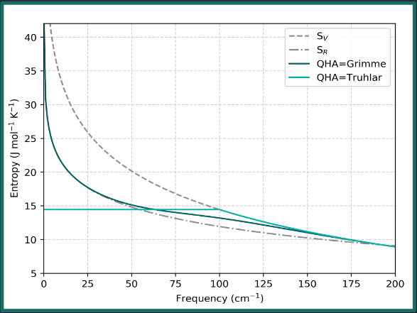
The quasi-harmonic correction has a greater effect when molecules have a greater number of low-frequency vibrational modes. For example:
Methylaniline: 2 vibrational modes below 200 cm-1
Int-III: 23 vibrational modes below 200 cm-1
goodvibes methylaniline.log Int-III.log
This gives the output:
o  Requested:

   Temperature = 298.15 Kelvin   Pressure = 1 atm
   All energetic values below shown in Hartree unless otherwise specified.
x  Caution! Different levels of theory found:
        -B97D/6-31G(d): methylaniline.log
        -wB97XD/Gen: Int-III.log

   Using vibrational scale factor 1.0: differing levels of theory detected.

   Caution! Implicit solvation (SMD/CPCM) detected. Enthalpic and entropic terms cannot be safely separated. Use them at your own risk!

   Entropic quasi-harmonic treatment: frequency cut-off value of 100.0 wavenumbers will be applied.
   QS = Grimme: Using a mixture of RRHO and Free-rotor vibrational entropies.
   REF: Grimme, S. Chem. Eur. J. 2012, 18, 9955-9964


   Structure                                           E        ZPE             H        T.S     T.qh-S          G(T)       qh-G(T)
   ********************************************************************************************************************************
o  methylaniline                             -326.664901   0.142118   -326.514489   0.039668   0.039535   -326.554157   -326.554024
o  Int-III                                  -8986.063880   0.446831  -8985.583025   0.106167   0.095367  -8985.689192  -8985.678393
   ********************************************************************************************************************************
Single Point Calculations
Useful for saving on computational resources:
We can optimize molecules at a lower level of theory to still obtain an accurate geometry, but do a single point energy calculation (SPC) at a higher level of theory to obtain more accurate energy values.
With the --spc argument, we can specify how the SPC file names are formatted.
Calculation Type |
Filename |
|---|---|
opt/freq |
file.log |
SPC |
file_SPC.log |
For example: ethane.log and ethane_TZ.out
goodvibes ethane.log --spc TZ
You will get the following output:
o  Requested: --spc TZ

   Temperature = 298.15 Kelvin   Pressure = 1 atm
   All energetic values below shown in Hartree unless otherwise specified.

o  Found vibrational scaling factor of 0.977 for B3LYP/6-31G(d) level of theory
   Alecu, I. M.; Zheng, J.; Zhao, Y.; Truhlar, D. G. J. Chem. Theory Comput. 2010, 6, 2872-2887.

   Entropic quasi-harmonic treatment: frequency cut-off value of 100.0 wavenumbers will be applied.
   QS = Grimme: Using a mixture of RRHO and Free-rotor vibrational entropies.
   REF: Grimme, S. Chem. Eur. J. 2012, 18, 9955-9964

   Combining final single point energy with thermal corrections.

   Structure                                       E_SPC             E        ZPE         H_SPC        T.S     T.qh-S      G(T)_SPC   qh-G(T)_SPC
   **********************************************************************************************************************************************
o  ethane                                     -79.858399    -79.830421   0.073508    -79.780448   0.027569   0.027570    -79.808017    -79.808019
   **********************************************************************************************************************************************
Warning
The --spc flag only contains the suffix used in the SPC filename. It is important that the
file name of the singlepoint calculation matches the optimization/frequency file name exactly,
except with the addition of the suffix after an underscore. The SPC suffix must also be the same
for all files in the folder – it will not work if some files have the suffix _SPC and others have _DLPNO.
Warning
When using the --spc flag, it is important that you don't call goodvibes
on the SPC files themselves, as the program will then look for a SPC for
the SPC file, which will not exist. The best way to work around this is to
use "opt" or "freq" or "calc" at the end of the original file names, then
use goodvibes *opt.log rather than *log to avoid this issue.
Potential Energy Surface Calculations:
GoodVibes can compute relative energy/thermochemistry values to describe a reaction pathway with a potential energy surface
To do this, we need to write a yaml file with 3 sections:
- PES
Defines reaction pathway
Can add multiple pathways
- SPECIES
Relates files to each species in the reaction pathway
- FORMAT
Optional additional formatting
--- # PES
    Ph: [Ph-Int1 , Ph-TS1 , Ph-Int2 , Ph-TS2 , Ph-Int3 ]
    Py: [Py-Int1 , Py-TS1 , Py-Int2 , Py-TS2 , Py-Int3 ]

--- # SPECIES
    Ph-Int1     : Int_I_Ph*
    Ph-TS1      : TS_1_Ph*
    Ph-Int2     : Int_II_Ph*
    Ph-TS2      : TS_II_Ph*
    Ph-Int3     : Int_III_Ph*
    Py-Int1     : Int_I_Py*
    Py-TS1      : TS_1_Py*
    Py-Int2     : Int_II_Py*
    Py-TS2      : TS_II_Py*
    Py-Int3     : Int_III_Py*

--- # FORMAT
    dec :  2
    legend : False
    color : black,#26a6a4
    pointlabel : False
    gridlines: True
    show_conformers: True
    show_gconf: False
    title: Potential Energy Surface
Note
The SPECIES section of the yaml file is where you define the files in the
directory that are to be assigned to each species in the reaction pathway.
In this example, the species Ph-Int1 is defined as all files that
begin with Int_I_Ph, as the wildcard * is used to ensure that all
files in a conformer ensemble are included in the calculations.
Tip
The --pes flag can be used any time you want to find a ∆G between two species or for a single
step in a reaction. You can specify
the "reaction" as only the two species of interest in order to find the relative energy between a
pair of conformer ensembles, provided the files for each species are in the same folder and start with
distinct names, allowing for correct identification in the SPECIES section of the yaml file.
Putting it All Together
Temperature adjustments
Single Point Calculations
Potential Energy Surface Calculations
We can use these 24 intermediate and transition state calculations + corresponding SPC files + yaml to define a reaction pathway
goodvibes *.log -t 353.15 --spc DLPNO --imag --invertifreq -5 --pes PhPy.yaml
You will get the following as output:
o  Requested: -t 353.15 --spc DLPNO --imag --invertifreq -5 --pes PhPy.yaml

   Temperature = 353.15 Kelvin   Pressure = 1 atm
   All energetic values below shown in Hartree unless otherwise specified.

   Using vibrational scale factor 1.0 for wB97XD/6-31+G(d) level of theory

   Caution! Implicit solvation (SMD/CPCM) detected. Enthalpic and entropic terms cannot be safely separated. Use them at your own risk!

   Entropic quasi-harmonic treatment: frequency cut-off value of 100.0 wavenumbers will be applied.
   QS = Grimme: Using a mixture of RRHO and Free-rotor vibrational entropies.
   REF: Grimme, S. Chem. Eur. J. 2012, 18, 9955-9964

   Combining final single point energy with thermal corrections.

   The following frequency was made positive and used in calculations: -2.8981 from Int_II_Py_b.log

   Structure                                       E_SPC             E        ZPE         H_SPC        T.S     T.qh-S      G(T)_SPC   qh-G(T)_SPC  im freq
   *******************************************************************************************************************************************************
o  Int_III_Ph_a                             -1414.272460  -1415.767800   0.418564  -1413.819815   0.105944   0.098578  -1413.925760  -1413.918394
o  Int_III_Py_a                             -1414.269254  -1415.765251   0.418693  -1413.816478   0.106976   0.099078  -1413.923454  -1413.915556
o  Int_III_Py_b                             -1414.270115  -1415.766283   0.417841  -1413.817909   0.107635   0.099479  -1413.925544  -1413.917389
o  Int_II_Ph_a                              -1414.238513  -1415.730395   0.418574  -1413.786351   0.102570   0.096587  -1413.888921  -1413.882937
o  Int_II_Py_a                              -1414.248486  -1415.739754   0.418595  -1413.796289   0.103963   0.097294  -1413.900253  -1413.893584
o  Int_II_Py_b                              -1414.251141  -1415.742543   0.418183  -1413.799010   0.107432   0.098914  -1413.906442  -1413.897924
o  Int_II_Py_c                              -1414.250426  -1415.740873   0.418274  -1413.798225   0.105693   0.098329  -1413.903918  -1413.896555
o  Int_I_Ph_a                               -1414.219198  -1415.708399   0.419425  -1413.766680   0.100260   0.095322  -1413.866940  -1413.862002
o  Int_I_Ph_b                               -1414.218356  -1415.706755   0.419581  -1413.765641   0.100615   0.095531  -1413.866255  -1413.861172
o  Int_I_Ph_c                               -1414.203378  -1415.689310   0.418363  -1413.751447   0.103593   0.097115  -1413.855040  -1413.848561
o  Int_I_Py_a                               -1414.223227  -1415.715045   0.419114  -1413.770810   0.101829   0.096167  -1413.872638  -1413.866977
o  Int_I_Py_b                               -1414.223209  -1415.711031   0.419045  -1413.770901   0.100816   0.095725  -1413.871717  -1413.866626
o  Int_I_Py_c                               -1414.211964  -1415.713255   0.418916  -1413.759687   0.101792   0.096060  -1413.861479  -1413.855747
o  Int_I_Py_d                               -1414.213688  -1415.698106   0.418680  -1413.761526   0.102616   0.096491  -1413.864142  -1413.858017
o  Int_I_Py_e                               -1414.212305  -1415.697383   0.418818  -1413.759995   0.103174   0.096642  -1413.863169  -1413.856637
o  Int_I_Py_f                               -1414.220429  -1415.706212   0.419258  -1413.767919   0.101285   0.095753  -1413.869204  -1413.863672
o  TS_1_Ph_a                                -1414.181410  -1415.670386   0.417010  -1413.731342   0.100555   0.095542  -1413.831896  -1413.826883  -523.12
o  TS_1_Ph_b                                -1414.173224  -1415.661334   0.416101  -1413.723679   0.102811   0.096739  -1413.826490  -1413.820418  -456.04
o  TS_1_Py_a                                -1414.194715  -1415.682140   0.417530  -1413.744164   0.100446   0.095392  -1413.844611  -1413.839556  -397.29
o  TS_1_Py_b                                -1414.199208  -1415.686916   0.417186  -1413.748822   0.101458   0.096001  -1413.850280  -1413.844823  -437.02
o  TS_1_Py_c                                -1414.192702  -1415.681170   0.416331  -1413.742779   0.103499   0.097006  -1413.846278  -1413.839786  -319.63
o  TS_II_Ph_a                               -1414.231879  -1415.727262   0.417335  -1413.781405   0.101901   0.095931  -1413.883306  -1413.877336  -241.51
o  TS_II_Py_a                               -1414.238504  -1415.734212   0.417525  -1413.787768   0.102732   0.096376  -1413.890500  -1413.884144  -200.84
o  TS_II_Py_b                               -1414.235758  -1415.731725   0.418091  -1413.784725   0.101249   0.095630  -1413.885974  -1413.880355  -239.51
   *******************************************************************************************************************************************************

   Gconf correction requested to be applied to below relative values using quasi-harmonic Boltzmann factors

   RXN: Ph (kcal/mol)                             DE_SPC            DE       DZPE        DH_SPC       T.DS    T.qh-DS      DG(T)_SPC   qh-DG(T)_SPC
   *******************************************************************************************************************************************************
o  Ph-Int1                                          0.00          0.00       0.00          0.00       0.00       0.00          0.00          0.00
o  Ph-TS1                                          23.56         23.54      -1.55         21.98      -0.31      -0.33         22.29         22.31
o  Ph-Int2                                        -12.29        -14.14      -0.57        -12.55       0.94       0.31        -13.49        -12.86
o  Ph-TS2                                          -8.13        -12.17      -1.34         -9.45       0.52      -0.10         -9.97         -9.35
o  Ph-Int3                                        -33.59        -37.61      -0.57        -33.55       3.05       1.56        -36.61        -35.11
   *******************************************************************************************************************************************************

   RXN: Py (kcal/mol)                             DE_SPC            DE       DZPE        DH_SPC       T.DS    T.qh-DS      DG(T)_SPC   qh-DG(T)_SPC
   *******************************************************************************************************************************************************
o  Py-Int1                                          0.00          0.00       0.00          0.00       0.00       0.00          0.00          0.00
o  Py-TS1                                          15.08         16.52      -1.20         13.83      -0.43      -0.46         14.27         14.29
o  Py-Int2                                        -17.45        -18.19      -0.55        -17.59       3.38       1.62        -20.97        -19.21
o  Py-TS2                                          -9.59        -13.17      -0.97        -10.61       0.35      -0.22        -10.96        -10.39
o  Py-Int3                                        -29.39        -33.24      -0.70        -29.44       3.60       1.91        -33.04        -31.35
   *******************************************************************************************************************************************************
Graphing these potential energy surfaces is simple once the yaml file is created
goodvibes *.log -t 353.15 --spc DLPNO --imag --invertifreq -5 --pes PhPy.yaml --graph PhPy.yaml
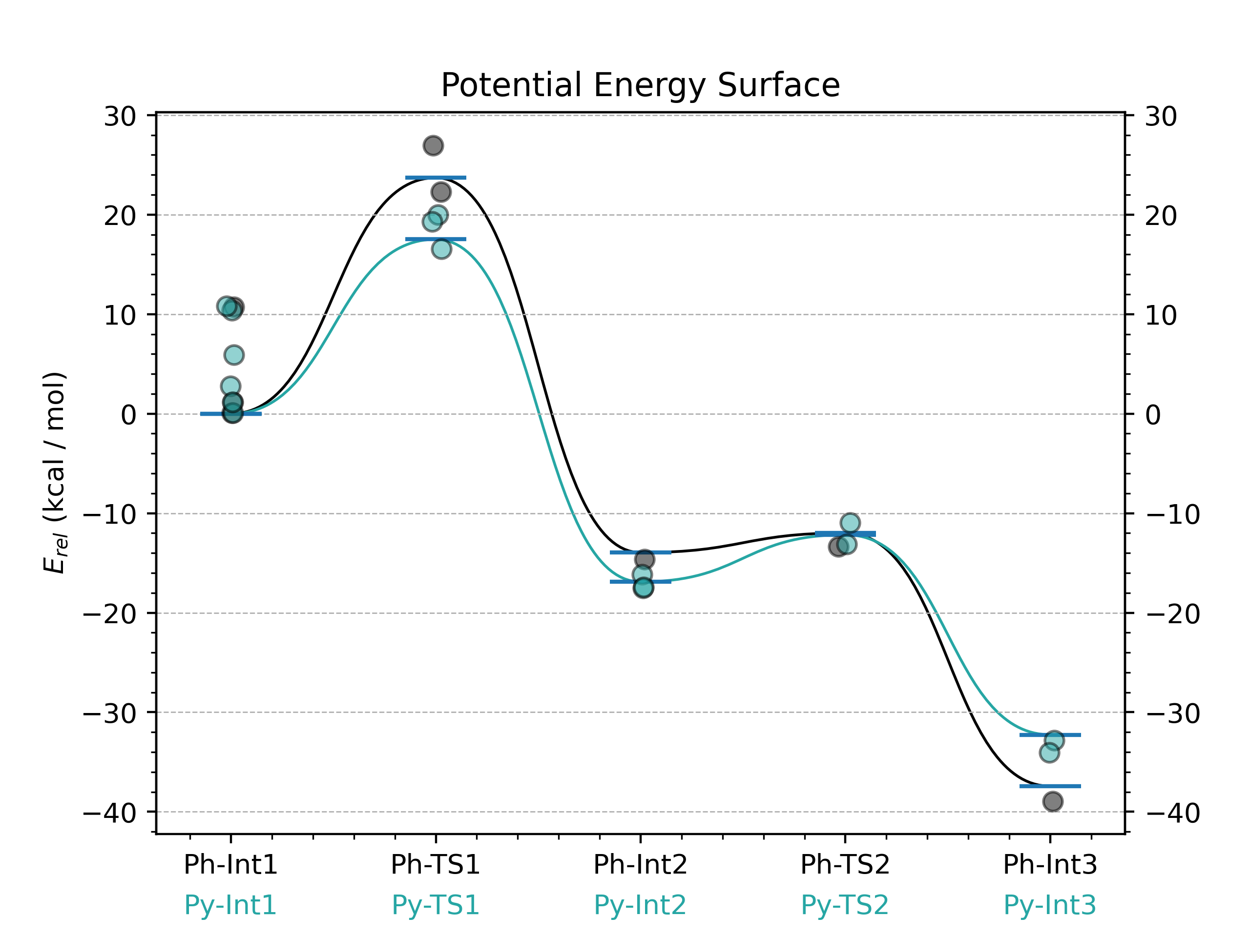
You can add more or less details by changing the FORMAT section of the yaml file. This is where you might tell GoodVibes you do not want to plot the different conformations of each structure, only the energies.
Running on Multiple Processors
GoodVibes allows you to run in multiple processors, reducing the wall time required for extracting the data.
This can be done with the --jobs flag:
goodvibes *.log --jobs 16
This will use 16 processors to run GoodVibes on all your Gaussian output files.
Saving Metadata
Another feature of GoodVibes is that it will save the metadata from a run in a JSON file.
This will allow users to add single point energy corrections, temperature corrections, concentration corrections, etc.
without needing to fully parse the data again. This is specified with the --json flag:
goodvibes *.log --json goodvibes_thermo_data.json
The JSON file contains the metadata for the run and can be called back in future runs with:
goodvibes --import goodvibes_thermo_data.json -t 310
Check out other packages by the Paton lab @ our GitHub!